Diffraction Limited PSF and MTF

In this example, we will show how to calculate the diffraction limited PSF and MTF for a circular aperture. We will also compare the numerically derived results from prysm with the analytical forms.

import numpy as np

from prysm import Pupil, PSF, MTF
from prysm.psf import airydisk
from prysm.otf import diffraction_limited_mtf

from matplotlib import pyplot as plt
%matplotlib inline
plt.style.use('bmh')

# system parameters
epd = 1
efl = 10
fno = efl / epd
wavelength = 0.5

p = Pupil(wavelength=wavelength, dia=epd, samples=256)
psf = PSF.from_pupil(p, efl)
u, sx = psf.slices().x

# calculate the analytical version, and the difference between the two
analytical_psf = airydisk(u, fno, wavelength)
psferr = (analytical_psf - sx)

fig, (ax1, ax2) = plt.subplots(ncols=2, figsize=(10,4))
psf.slices().plot('x', fig=fig, ax=ax1, xlim=50)
ax1.plot(u, analytical_psf, ls=':', c='k', label='Analytic', zorder=3)
ax1.legend()
ax2.plot(u, psferr, lw=3)
ax2.set(xlim=(-50,50), xlabel=r'Image Plane X [$\mu m$]', ylabel='Intensity Difference an - numerical')
fig.tight_layout()

/home/docs/checkouts/readthedocs.org/user_builds/prysm/envs/v0.19/lib/python3.7/site-packages/prysm/mathops.py:33: RuntimeWarning: invalid value encountered in true_divide
  out = special_engine.j1(r) / r

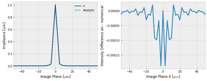
One can see that the differences manifest below the fourth decimal place. It might be interesting to see the RMS error,

from prysm.util import rms

rms(psferr)

1.4915844378638162e-05

This error is over a 1D slice. If calculated over the whole image plane it would be much smaller.

Next, we consider the MTF:

# calculate the MTF and its error
mtf = MTF.from_psf(psf)
nu, m = mtf.slices().x
m_analytic = diffraction_limited_mtf(fno, wavelength, frequencies=nu)
mtferr = (m_analytic - m)

fig, (ax1, ax2) = plt.subplots(ncols=2, figsize=(10,4))
mtf.slices().plot('x', fig=fig, ax=ax1)
ax1.plot(nu, m_analytic, ls=':', c='k', label='Analytic', zorder=3)
ax1.legend()
ax2.plot(nu, mtferr, lw=3)
ax2.set(xlim=(0,200), ylim=(-0.0005,0.0005), xlabel='Spatial Frequency [cy/mm]', ylabel='MTF Difference [a.u.]')
fig.tight_layout()

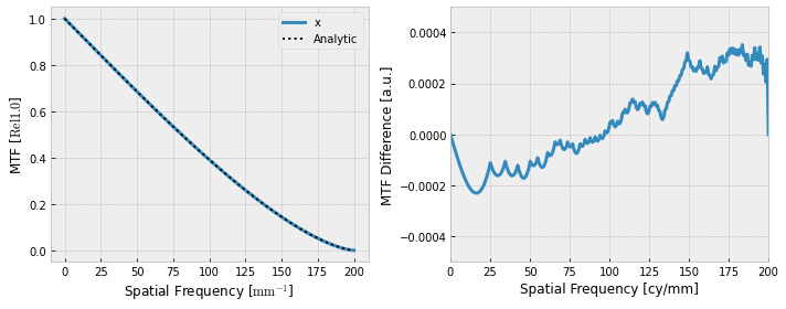
Once again the error is at the fourth decimal place. The RMS may be interesting again,

rms(mtferr)

0.00018149825282460713